Analyzing the Stroop Effect,
Udacity, Data Analyst Nanodegree, Project: Test a perceptual Phenomenon
Praxitelis-Nikolaos Kouroupetroglou
Introduction
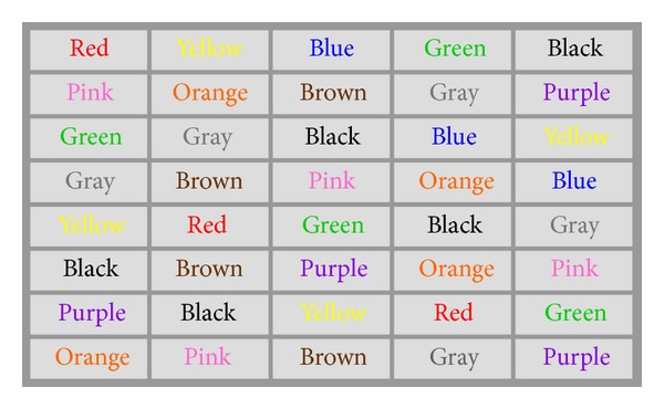
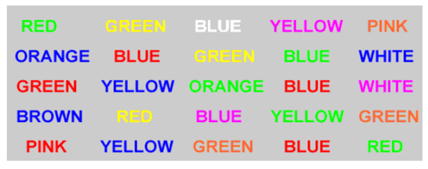
This project explore the Stroop Effect, The Stroop Effect is named by the John Ridley Stroop who first published the effect in English in 1935. In summary this effect explores has 2 experiments, the first one measures the time it takes for an individual to identify the name of a color (e.g., "blue", "green", or "red") that is printed in a color which that is denoted by its name (for example, the word "blue" printed in blue), and the second experiment measures the time it take for an individual to identify the name of a color that is printed in a color which is not denoted by its name (for example, the word "blue" printed in red and not in blue). naming the color of the word takes longer and is more prone to errors than when the color of the ink matches the name of the color reference.
This project comes with a dataset in csv format which can be found in this link. The dataset contains 2 colunms which contains the time it took to a sample of people to finish the Stroop Effect test to identify to color name. The dataset has 2 columns; the first one is called "Conguent" which contains the time it took to each participant to identify the color names which matched to the printed text and the second one is called "Inconguent" which means the time it took to each participant to indentify the name of the color which did not match to the printed text reference.
Congruent Colors and Words example:

Incongruent Colors and Words example:

What is the independent variable? What is the dependent variable?
Independent variable : Word Condition (Congruent or Incongruent) Dependent variable : the time it takes to name the colors
What is an appropriate set of hypotheses for this task? What kind of statistical test do you expect to perform? Justify your choices.
Null Hypothesis ( $H_{0}:\mu_{1}=\mu_{2}$) The average time that it takes to identify a color is the same for the two groups (congruent color with word and incongruent color with word) at alpha level of a = 0.05 .
Alternative Hypothesis ( $H_{1}:\mu_{1}\ne\mu_{2}$) The average time that it takes to identify a color is not same for the two groups (congruent color with word and incongruent color with word) at alpha level of a = 0.05 .
Type of Statistical Test : dependent t-test (two tailed), It must be compared that the means of two related groups to determine the statistical significant difference between two means. we can assume normal distribution to the two groups, and it has to be two tailed because our hypothesis is testing equality of two means. Furthermore, we don't have any population parameters, thus a z-test would not fit to examine this phenomenon.
Exploring the dataset
Lets begin exploring the 2 groups:
#import libraries
import pandas as pd
import seaborn as sns
import numpy as np
import matplotlib.pyplot as plt
%matplotlib inline
# read csv file and save to df
df = pd.read_csv('stroopdata.csv')

# csv head
print(df.head(7))

# csv summary
df.describe()
At first glance, the 2 experiments so some differences, the experiment for congruent color and text has mean value equal to 14.05 and the other one has 22.01 which differ more than the other. In general the second experiment (Incongruent) declines from the first one (Congruent), as we can see the standard deviation, the 1st quantile, the 3rd quantile, min and max are larger than the first group.
Univariate Plots
Lets plot the histogram of the 2 groups
Congruent Experiment Histogram:
# Congruent colors and words histogram
fig, ax = plt.subplots()
sns.distplot(df['Congruent'], color="blue", kde=False)
ax.set_xlabel("time")
ax.set_ylabel("count")
ax.set_title("Congruent Histogram")
Incongruent Experiment Histogram:
# Incongruent colors and words histogram
fig, ax = plt.subplots()
sns.distplot(df['Incongruent'], color="orange", kde=False)
ax.set_xlabel("time")
ax.set_ylabel("count")
ax.set_title("Incongruent Histogram")
Bivariate Plots
# Congruent and Incongruent colors and words boxplots
fig, ax = plt.subplots()
sns.boxplot(data=df)
ax.set_title("Congruent, Incongruent Boxplots")
By inspecting at the boxplot, we can see that the average completion time of Incongruent group is higher. The box plot also shows that the incongruent group has two outliers.
# Congruent colors and words histograms side by side
fig, ax = plt.subplots()
sns.distplot( df["Congruent"] , color="blue", kde=False)
sns.distplot( df["Incongruent"] , color="orange", kde=False)
ax.set_xlim([0, 45])
ax.set_xlabel("time")
ax.set_ylabel("count")
ax.set_title("Congruent, Incongruent Distributions")
The distribution for both congruent and incongruent group looks normal.
Performing a statistical test
# Performing the statistical test
from scipy import stats

n = df.Congruent.count()
degrees_of_Freedom = n - 1
alpha = 0.05
print("size of samples", n)
print("degrees of freedom:", degrees_of_Freedom)
print("alpha level: ", alpha)

t_critical = np.round(-1 * stats.t.ppf(alpha/2, degrees_of_Freedom), 3)
print("t-critical value from a = 0.05 for two tailed test:", t_critical)


# Calculates the T-test for the two related samples of scores, a and b.
res = stats.ttest_rel(df['Incongruent'], df['Congruent'])
t_statistic = round(res[0], 3)
p_value = round(res[1], 8)
print("t-statistic:", t_statistic)
print("p-value:", p_value)
p value is far below the p value for the critical region which is 0.025 therefore, we reject the null hypothesis. Hence, we can conclude that incongruent group and congruent group has a significant difference between them and there is a different average population time to identify colors.
Lets continue investigate even further this phenomenon:
## step by step computations

# calculate the point of interest
point_of_interest = np.round(df.Incongruent.mean() - df.Congruent.mean(), 3)
print("point of interest:", point_of_interest)

# calculate the standard error of the difference
std_error = np.round(np.sqrt(np.sum((df.Incongruent - df.Congruent - point_of_interest)**2)/degrees_of_Freedom), 3)
print("standard error:", std_error)

# calculate the margin of error
margin_of_error = np.round(t_critical * std_error, 3)
print("margin of error:", margin_of_error)

# compute manually the t-statistic, t = Point_of_interest/(std_error/√n)
t_statistic_manually_computed = np.round(point_of_interest/(std_error/np.sqrt(df.Congruent.count())), 3)
print("t-statistic:", t_statistic_manually_computed)

# compute the Confidence Interval
lower_bound = np.round(point_of_interest - (t_critical * (std_error/np.sqrt(n))), 3)
upper_bound = np.round(point_of_interest + (t_critical * (std_error/np.sqrt(n))), 3)
print("Conffidence Interval: (", lower_bound, ",", upper_bound, ")")
After the manual computations, and here the t-statistic is 8.021 which is greater than t-critical value which is 2.069, hence as we applied and in the previous code snippet with the p-value and here we reject the null hypothesis.
Possible Cause of Effect Observed
I believe that sometimes for the general public is easier to identify colors written in their own name with the same color. However it is harder and very confusing to identify a color in a word that is colored with a different.